Application of Derivatives Class 12 Notes For Maths Chapter 6

NCERT Notes for Class 12 Mathematics

Chapter 6: Application of Derivatives

Tangents and Normals

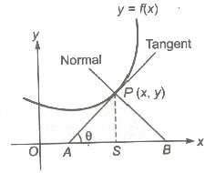
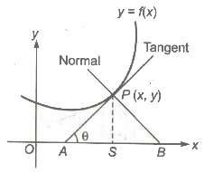
The derivative of the curve y = f(x) is f ‗(x) which represents the slope of tangent and equation of the tangent to the curve at P is

where (x, y) is an arbitrary point on the tangent.

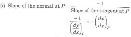
The equation of normal at (x, y) to the curve is

1. Ifthen the equations of the tangent and normal at (x, y) are (Y – y) = 0 and (X – x) = 0, respectively.
2. Ifthen the equation of the tangent and normal at (x, y) are (X – x) = 0 and (Y – y) = 0, respectively.

Slope of Tangent

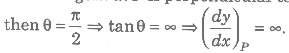
(i) If the tangent at P is perpendicular to x-axis or parallel to y-axis,

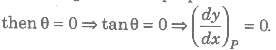
(ii) If the tangent at P is perpendicular to y-axis or parallel to x-axis,

Slope of Normal

(ii) If, then normal at (x, y) is parallel to y-axis and perpendicular to x-axis.

(iii) Ifthen normal at (x, y) is parallel to x-axis and perpendicular to y-axis.

Length of Tangent and Normal

(i) Length of tangent, PA = y cosec θ =

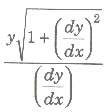
(ii) Length of normal,

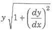
(iii) Length of subtangent,

(iv) Length of subnormal,

Angle of Intersection of Two Curves

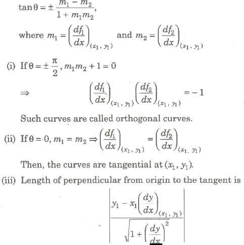
Let y = f₁(x) and y = f₂(x) be the two curves, meeting at some point P (x₁, y₁), then the angle between the two curves at P (x₁, y₁) = The angle between the tangents to the curves at P (x₁, y₁)

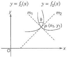
The other angle between the tangents is (180 — θ). Generally, the smaller of these two angles is taken to be the angle of intersection.
∴ The angle of intersection of two curves θ is given by

Derivatives as the Rate of Change

If a variable quantity y is some function of time t i.e., y = f(t), then small change in Δt time At have a corresponding change Δy in y.
Thus, the average rate of change = (Δy/Δt)
When limit At Δt→ 0 is applied, the rate of change becomes instantaneous and we get the rate of change with respect to at the instant x.

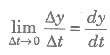
So, the differential coefficient of y with respect to x i.e., (dy/dx) is nothing but the rate of increase of y relative to x.

Rolle’s Theorem

Let f be a real-valued function defined in the closed interval [a, b], such that

1. f is continuous in the closed interval [a, b].
2. f(x) is differentiable in the open interval (a, b).
3. f(a)= f(b)

Then, there is some point c in the open interval (a, b), such that f‘ (c) = 0.

Geometrically Under the assumptions of Rolle‘s theorem, the graph of f(x) starts at point (a, 0) and ends at point (b, 0) as shown in figures.

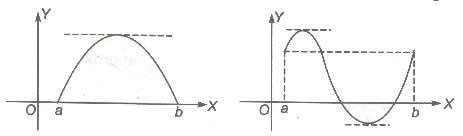
The conclusion is that there is at least one point c between a and b, such that the tangent to the graph at (c, f(c)) is parallel to the x-axis.

Algebraic Interpretation of Rolle’s Theorem

Between any two roots of a polynomial f(x), there is always a root of its derivative f‘ (x).

Lagrange’s Mean Value Theorem

Let f be a real function, continuous on the closed interval [a, b] and differentiable in the open interval (a, b). Then, there is at least one point c in the open interval (a, b), such that

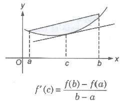
Geometrically Any chord of the curve y = f(x), there is a point on the graph, where the tangent is parallel to this chord.
Remarks In the particular case, where f(a) = f(b).
The expression [f(b) – f(a)/(b – a)] becomes zero. Thus, when
f(a) = f (b), f ‗ (c) = 0 for some c in (a, b).
Thus, Rolle‘s theorem becomes a particular case of the mean value theorem.

Approximations and Errors

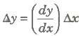
1. Let y = f(x) be a given function. Let Ax denotes a small increment in Δx, corresponding which y increases by Δy. Then, for small increments, we assume that

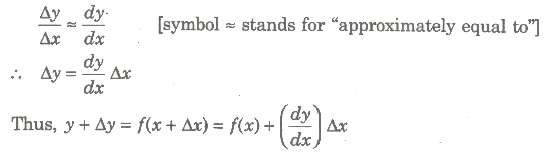
2. Let Δx be the error in the measurement of independent variable x and Δy is corresponding error in the measurement of dependent variable y. Then,

• Δy = Absolute error in measurement of y
• (Δy/y) = Relative error in measurement of y
• (Δy/y) * 100 = Percentage error in measurement of y

Monotonicity of Functions

1. Monotonic Function

A function f(x) is said to be monotonic on an interval (a, b), if it is either increasing or decreasing on (a, b).

2. Strictly Increasing Function

f(x) is said to be increasing in D1, if for every x1, x2 ∈ D1, x1 > x2 ⇒ f(x1) > f(x2). It means that there is a certain increase in the value of f(x) with an increase in the value of x.

3. Classification of Strictly Increasing Function

4. Non-Decreasing Function

f(x) is said to be non-decreasing in D1, if for every x1, x2 ∈ D1, x1 > x2 ⇒ f(x1) ≥ f(x2). It means that the value of f(x) would new decrease with an increase in the value of x.

5. Strictly Decreasing Function

f(x) is said to be decreasing in D1, if for every x1, x2 ∈ D1, x1 > x2 ⇒ f(x1) < f(x2). It means that there is a certain decrease in the value c f(x) with an increase in the value of x.

Classification of Strictly Decreasing Function

6. Non-increasing Function

f(x) is said to be non-increasing in D₁, if for every x₁, x₂ ∈ D₁, x₁ > x₂ ⇒ f(x₁) ≤ f(x₂). It means that the value of f(x) would never increase with an increase in the value of x.
If a function is either strictly increasing or strictly decreasing, then it is also a monotonic function.

Important Points to be Remembered

(i) A function f (x) is said to be increasing (decreasing) at point x₀, if there is an interval (x₀ — h, x₀ + h) containing x₀, such that f(x) is increasing (decreasing) on (x₀ — h, x₀ + h).
(ii) A function f (x) is said to be increasing on [a , b], if it is increasing (decreasing) on (a ,b) and it is also increasing at x = a and x = b.
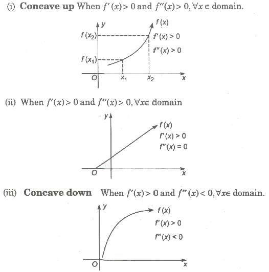
(iii) If (x) is increasing function on (a , b), then tangent at every point on the curve y = f(x) makes an acute angle θ with the positive direction of x-axis.

(iv) Let f be a differentiable real function defined on an open interval (a, b).
• If f ‗ (x) > 0 for all x ∈ (a, b), then f (x) is increasing on (a, b).
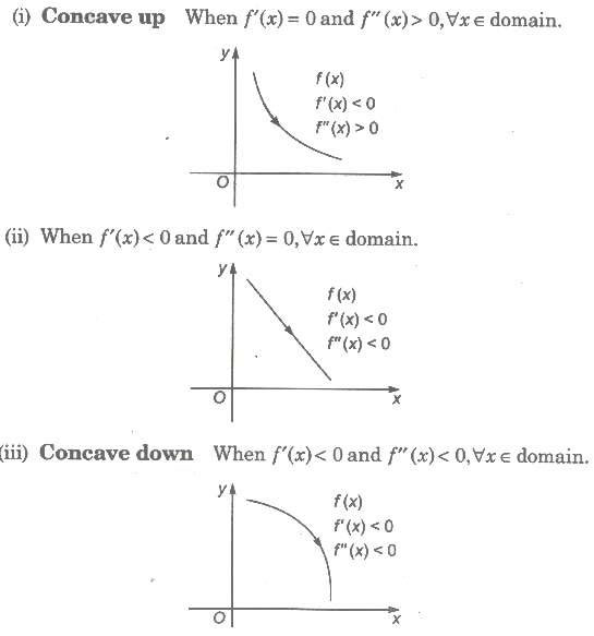
• If f ‗ (x) < 0 for all x ∈ (a , b), then f (x) is decreasing on (a, b).

(v) Let f be a function defined on (a, b).
• If f ‗(x) > 0 for all x ∈ (a, b) except for a finite number of points, where f ‗ (x) = 0, then f(x) is increasing on (a, b).
• If f ‗(x) < 0 for all x ∈ (a , b) except for a finite number of points, where f ‗(x) = 0, then f(x) is decreasing on (a , b).

Properties of Monotonic Functions

1. If f(x)is strictly increasing function on an interval [a, b], then f-1 exist and also a strictly increasing function.
2. If f(x) is strictly increasing function on [a, b], such that it is continuous, then f-1 is continuous on [f(a), f(b)].
3. If f(x) and g(x) are strictly increasing (or decreasing) function on [a, b], then gof(x) is strictly increasing (or decreasing) function on [a, b].
4. If one of the two functions f(x) and g(x) is strictly increasing and other a strictly decreasing, then gof(x) is strictly decreasing on [a, b].
5. If f(x) is continuous on [a, b], such that f‘ (c) ≥ 0 (f ‗ (c) > 0) for each c ∈ (a, b) is strictly increasing function on [a, b].
6. If f(x) is continuous on [a, b] such that f ‗(c) ≤ (f ‗ (c) < 0) for each c ∈ (a, b), then f(x) is strictly decreasing function on [a, b].

Maxima and Minima of Functions

1. A function y = f(x) is said to have a local maximum at a point x = a. If f(x) ≤ f(a) for all x ∈ (a – h, a + h), where h is somewhat small but positive quantity.

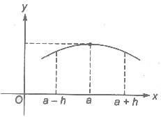
The point x = a is called a point of maximum of the function f(x) and f(a) is known as the maximum value or the greatest value or the absolute maximum value of f(x).

2. The function y = f(x) is said to have a local minimum at a point x = a, if f(x) ≥ f(a) for all x ∈ (a – h, a + h), where h is somewhat small but positive quantity.

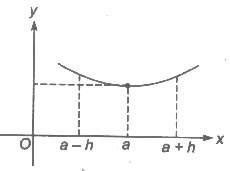
The point x = a is called a point of minimum of the function f(x) and f(a) is known as the minimum value or the least value or the absolute minimum value of f(x).

Properties of Maxima and Minima

1. If f(x) is continuous function in its domain, then at least one maxima and one minima must lie between two equal values of x.
2. Maxima and minima occur alternately, i.e., between two maxima there is one minima and vice-versa.
3. If f(x) → ∞ as x → a or b and f ‗ (x) = 0 only for one value of x (sayc) between a and b, then f(c) is necessarily the minimum and the least value.
4. If f(x) → p -∞ as x → a or b and f(c) is necessarily the maximum and the greatest value.

Important Points to be Remembered

1. If f(x) be a differentiable functions, then f ‗(x) vanishes at every local maximum and at every local minimum.
2. The converse of above is not true, i.e., every point at which f‘ (x) vanishes need not be a local maximum or minimum. e.g., if f(x) = x³ then f ‗(0) = 0, but at x =0. The function has neither minimum nor maximum. In general these points are point of inflection.
3. A function may attain an extreme value at a point without being derivable there at, e.g., f(x) = |x| has a minima at x = 0 but f’(0) does not exist.
4. A function f(x) can has several local maximum and local minimum values in an interval. Thus, the maximum and minimum values of f(x) defined above are not necessarily the greatest and the least values of f(x) in a given interval.
5. A minimum value at some point may even be greater than a maximum values at some other point.

Maximum and Minimum Values in a Closed Interval

Let y = f(x) be a function defined on [a, b]. By a local maximum (or local minimum) value of a function at a point c ∈ [a, b] we mean the greatest (or the least) value in the immediate neighbourhood of x = c. It does not mean the greatest or absolute maximum (or the least or absolute minimum) of f(x) in the interval [a, b].
A function may have a number of local maxima or local minima in a given interval and even a local minimum may be greater than a relative maximum.

Local Maximum

A function f(x) is said to attain a local maximum at x = a, if there exists a neighbourhood (a – δ, a + δ), of c such that, f(x) < f(a), ∀ x ∈ (a – δ, α + δ), x ≠ a or f(x) – f(a)< 0, ∀ x ∈ (a – δ, α + δ), x ≠ a
In such a case f(a) is called to attain a local maximum value of f(x) at x = a.

Local Minimum

f (x) > f(a), ∀ x ∈ (a – δ, α + δ), x ≠ a or f(x) – f(a) > 0, ∀ x ∈ (a – δ, α + δ), x ≠ a
In such a case f(a) is called the local minimum value of f(x) at x = a.

Methods to Find Local Extremum

1. First Derivative Test

Let f(x) be a differentiable function on an interval I and a ∈ I. Then,

1. (i) Point a is a local maximum of f(x), if
(a) f ‗(a) = 0
(b) f ‗(x) > 0, if x ∈ (a – h, a) and f‘ (x) < 0, if x ∈ (a, a + h), where h is a small but positive quantity.

2. (ii) Point a is a local minimum of f(x), if
(a) f ‗(a) = 0
(b) f ‗(a) < 0, if x ∈ (a – h, a) and f ‗(x) > 0, if x ∈ (a, a + h), where h is a small but positive quantity.

3. (iii) If f ‗(a) = 0 but f ‗(x) does not changes sign in (a – h, a + h), for any positive quantity h, then x = a is neither a point of minimum nor a point of maximum.

2. Second Derivative Test

Let f(x) be a differentiable function on an interval I. Let a ∈ I is such that f ―(x) is continuous at x = a. Then,

1. x = a is a point of local maximum, if f ‗(a) = 0 and f ―(a) < 0.
2. x = a is a point of local minimum, if f ‗(a) = 0 and f‖(a) > 0.
3. If f ‗(a) = f ―(a) = 0, but f‖ (a) ≠ 0, if exists, then x = a is neither a point of local maximum nor a point of local minimum and is called point of inflection.
4. If f ‗(a) = f ―(a) = f ‗‖(a) = 0 and f ^iv(a) < 0, then it is a local maximum. And if f ^iv > 0, then it is a local minimum.

nth Derivative Test

Let f be a differentiable function on an interval / and let a be an interior point of / such that

(i) f ‗(a) = f ―(a) = f ‗‖(a) = … f ^{n – 1}(a) = 0 and
(ii) fn (a) exists and is non-zero, then
• If n is even and f ⁿ (a) < 0 ⇒ x = a is a point of local maximum.
• If n is even and f ⁿ (a) > 0 ⇒ x = a is a point of local minimum.
• If n is odd ⇒ x = a is a point of local maximum nor a point of local minimum.

Important Points to be Remembered

1. To Find Range of a Continuous Function Let f(x) be a continuous function on [a, b], such that its least value in [a, b1 is m and the greatest value in [a, b] is M. Then, range of value of f(x) for x ∈ [a, b] is [m, M].
2. To Check for the injectivity of a Function A strictly monotonic function is always oneone (injective). Hence, a function f (x) is one-one in the interval [a, b], if f ‗(x) > 0 , ∀ x ∈ [a, b] or f‘ (x) < 0 , ∀ x ∈ [a, b].
3. The points at which a function attains either the local maximum value or local minimum values are known as the extreme points or turning points and both local maximum and local minimum values are called the extreme values of f(x). Thus, a function attains an extreme value at x = a, if f(a) is either a local maximum value or a local minimum value. Consequently at an extreme point ‗a‘, f (x) — f (a) keeps the same sign for all values of x in a deleted nbd of a.
4. A necessary condition for (a) to be an extreme value of a function (x) is that f ‗(a) = 0 in case it exists.
5. This condition is only a necessary condition for the point x = a to be an extreme point. It is not sufficient. i.e., f ‗(a) = 0 does not necessarily imply that x = a is an extreme point.
There are functions for which the derivatives vanish at a point but do not have an extreme value. e.g., the function f(x) = x³ , f ‗(0) = 0 but at x = 0 the function does not attain an extreme value.
6. Geometrically the above condition means that the tangent to the curve y = f(x) at a point where the ordinate is maximum or minimum is parallel to the x-axis.
7. All x,for which f ‗(x) = 0, do not give us the extreme values. The values of x for which f ‗(x) = 0 are called stationary values or critical values of x and the corresponding values of f(x) are called stationary or turning values of f(x).

Critical Points of a Function

Points where a function f(x) is not differentiable and points where its derivative (differentiable coefficient) is z ?,ro are called the critical points of the function f(x).

Maximum and minimum values of a function f(x) can occur only at critical points. However, this does not mean that the function will have maximum or minimum values at all critical points. Thus, the points where maximum or minimum value occurs are necessarily critical Points but a function may or may not have maximum or minimum value at a critical point.

Point of Inflection

Consider function f(x) = x³. At x = 0, f ‗(x)= 0. Also, f ―(x) = 0 at x = 0. Such point is called point of inflection, where 2nd derivative is zero. Consider another function f(x) = sin x, f ―(x)= – sin x. Now, f ―(x)= 0 when x = nπ, then this points are called point of inflection.

At point of inflection

1. It is not necessary that 1st derivative is zero.
2. 2^nd derivative must be zero or 2nd derivative changes sign in the neighbourhood of point of inflection.

Concept of Global Maximum/Minimum

• Let y = f(x) be a given function with domain D.
• Let [a, b] ⊆ D, then global maximum/minimum of f(x) in [a, b] is basically the greatest/least value of f(x) in [a, b].
• Global maxima/minima in [a, b] would always occur at critical points of f(x) with in [a, b] or at end points of the interval.

Global Maximum/Minimum in [a, b]

In order to find the global maximum and minimum of f(x) in [a, b], find out all critical points of f(x) in [a, b] (i.e., all points at which f ‗(x)= 0) and let f(c₁), f(c₂) ,…, f(_n) be the values of the function at these points.

Then, M₁ → Global maxima or greatest value. and M₁ → Global minima or least value.
where M₁ = max { f(a), f(c₁), f(c₁) ,…, f(c_n), f(b)} and M₁ = min { f(a), f(c₁), f(c₂) ,…, f(c_n), f(b)}

Then, M₁ is the greatest value or global maxima in [a, b] and M₁ is the least value or global minima in [a, b].

Ncert Solution for class 6 to 12 download in pdf